Adv Calc Outline

GO

Limits of Multivariate Functions §

• We may approach a point in 3D space from infinitely many paths, from infinitely many directions and angles
• To prove that the limit does not exist, only need to find a counterexample: 2 paths in which the limit differ
• There are a few simple and common limits we can test first

Procedure: Counterexample Path Tests §

Straight Line Test §

• This checks the limit approached by all straight lines to the target point
  • Check for approaching from $x-$axis: $x\to 0,y=0$
  • Check for approaching from $y-$axis: $x=0,r\to 0$
  • Check for general equation of a line: $y=mx$
• Replace the limit equation with the new values

Parabolic Line Test §

• This checks the limit approached by all parabolic paths to the target point
  • Check for approaching from vertically-opening parabola: $y=m{x}^2$
  • Check for approaching from horizontally-opening parabola: $x=m{y}^2$

Procedure: Polar / Lasso Test §

• If the limit exists, no matter what kind of path approaches our point, the distance to the point, $r$, will approach 0. This motivates the polar definition

$$(x,y)\to (0,0)\Rightarrow r\to 0^{+}$$

1. Convert the variables of the limit from $(x,y)$ form to $(r,\varphi )$ form
2. Convert all $x,y$ in the function into $r\cos \varphi ,r\sin \varphi$
3. Simplify and evaluate; ensure that the final expression will not go to infinity or undefined

Example: Limit Testing with Polar Coordinates

Given function $f=\frac{3x^{2}y}{x^2+y^2}$, determine whether the limit exists at $(0,0)$.

$$\begin{array}{rlr}& \underset{(x,y)\to (0,0)}{\lim }\frac{3x^{2}y}{x^2+y^2}& \\ =& \underset{(r,\varphi )\to (0^{+},0)}{\lim }\frac{3(r\cos \varphi {)}^2\cdot r\sin \varphi }{r{\cos }^2\varphi \cdot r{\sin }^2\varphi }& \text{Polar representation}\\ =& \underset{(r,\varphi )\to (0^{+},0)}{\lim }\frac{3r^3\cdot \sin \varphi \cdot {\cos }^2\varphi }{r^2}& \\ =& \underset{(r,\varphi )\to (0^{+},0)}{\lim }3r\underset{\text{Bounded from [-1,1]}}{\underbrace{\cdot \sin \varphi \cdot {\cos }^2\varphi }}& \\ =& 0& \end{array}$$

Note that it is necessary to check that the final expression is bounded, and will not "blow up" to infinity or undefined. Therefore, this means that for all paths and angles on the graph of $f(x,y)$ approaching $(0,0)$, the limit is defined.

Tangent Planes and Normal Lines to Smooth Function in 3D space §

Procedure: Finding a Tangent Plane given a Function and Point §

• Tangent planes are used to approximate the behaviour of our multivariate function
• Given a function $f(x,y)$ and a point $P(x_0,y_0)$, we find thee equation of the planet tangent to that point by

$$z=\frac{\partial f}{\partial x}(x_0,y_0)\cdot (x-x_0)+\frac{\partial f}{\partial y}(x_0,y_0)\cdot (y-y_0)+f(x_0,y_0)$$

Example: Finding Tangent Plane given Function and Point

Find the equation of the tangent plane to $f(x,y)$ to $f(x,y)=\frac{x}{y^2+1}$ at point $P(2,1)$.

Linear Approximation and Differentials §

Procedure: Linear Approximation §

• Given a function $f(x,y)$ and point $P(x_0,y_0)$ and asked to approximate the value at $P$, we conceive a more convenient point $(a,b)$ for evaluating and the linear approximation is

$$L(x,y)=\frac{\partial f}{\partial x}(a,b)\cdot (x_0-a)+\frac{\partial f}{\partial y}(a,b)\cdot (y_0-b)+f(a,b)$$

Procedure: Differentials §

• The small incremented difference between $f(a,b)$ and the amount added to it

$$\begin{array}{rl}\Delta f& =\frac{\partial f}{\partial x}dx+\frac{\partial f}{\partial y}dy\\ \Delta f(x,y)& =\frac{\partial f}{\partial x}(a,b)\cdot (x_0-a)+\frac{\partial f}{\partial y}(a,b)\cdot (y_0-b)\end{array}$$

Example: Linear Approximation and Differentials

Given function $f(x,y)=5x^2\cdot \sqrt{x^2+y^2}-100$, estimate $f(2.9,4.2)$ and compute the resulting differential.

Chain Rule for Paths §

Procedure: Chain Rule for Paths §

• When asked to solve the derivative of a function to a variable, through which there are “intermediate variables” present, we may use the chain rule for paths.
• For a function $f(x,y)$, where $x=g(t)$ and $y=h(t)$, $\frac{\partial f}{\partial t}$ can be given by the following tree diagram and equation:

$$\frac{\partial f}{\partial t}=\frac{\partial f}{\partial x}\frac{dx}{dt}+\frac{\partial f}{\partial y}\frac{dy}{dt}$$

Note

If a function has only one variable, then we express it as the derivative. If a function has more than one variable, than express it as the partial derivative

Directional Derivatives and Gradient §

Procedure: Directional Derivatives §

• Imagine that we are a bug travelling along a very short path over a function
• We may find the rate of change of a function $f(x,y)$ at the point $(a,b)$ along vector path $\vec{u}$, where $\vec{u}$ is a unit vector, using directional derivatives:

$$D\vec{u}f(a,b)=\frac{\partial f}{\partial x}(a,b)\overrightarrow{u_1}+\frac{\partial f}{\partial y}(a,b)\overrightarrow{u_2}$$

Unitising the vector Given a generic direction vector $\vec{u}$, we unitise the vector by dividing it by its magnitude: $\vec{u}=\frac{\vec{v}}{||\vec{v}||}$

Example: Directional Derivatives

Let us have function $f(x,y,z)=y\cdot ln(1+x^2)+\arctan (z)$ at point $P(0,1,1)$ and directional vector $\overrightarrow{pq}$, where $p=⟨0,1,1⟩$, and $q=⟨-1,-1,3⟩$

Find unit vector $\vec{u}$: $\overrightarrow{q-p}=⟨-1,-2,2⟩$

Unitise vector: $\vec{u}=\frac{⟨-1,-2,2⟩}{3}=⟨-\frac{1}{3},\frac{-2}{3},\frac{2}{3}⟩$

Find partial derivatives: $\frac{\partial f}{\partial x}$ = $\frac{\partial f}{\partial y}$ =

Local and Global Extrema §

Unconstrained extrema §

• Find critical points
• Find discriminant for each point $D(x_0,y_0)=\frac{{\partial }^{2}f}{\partial x^2}\cdot \frac{\partial f^2}{\partial y^2}-{\left(\frac{{\partial }^{2}f}{\partial x\partial y}\right)}^2$
• Use the following criteria to analyse the result:

Discriminant	Value of $\frac{{\partial }^{2}f}{\partial x^2}$	Result
0		Undetermined
Smaller than 0		Saddle Point
Larger than 0	Larger than 0	Local min
Larger than 0	Smaller than 0	Local max

Constrained extrema §

• The criteria for finding global extrema for multivariate functions is very similar to the criteria for single-variable calculus
• If $D$ is a closed and bounded set in ${\mathbb{R}}^2$, and $f:D\to \mathbb{R}$ is continuous:
  1. $f$ attains a global maximum and global minimum in $D$, and
  2. The global extreme occur at critical points or along the boundary of $D$
• It’s very important that $D$ is bounded; otherwise it may be impossible to find extrema
• We may use two techniques for finding extrema along boundary $D$ in a systematic manner

Case 1: Function bounded by region defined by points §

Procedure: Boundary Graphs §

• To find the global extrema of a continuous function $f$ over a closed, bounded $D$:
  1. Find critical points of $f$ in $D$ by computing the partial derivatives in respect to each variable, and setting system of equations where $\frac{\partial f}{\partial x}=0$ and $\frac{\partial f}{\partial y}=0$
  2. Draw a 2-d boundary graph lying on the $xy$ plane for the restricted points
  3. Analyse each side of the boundary graph to determine extreme values of $f$ on the boundary of $D$
  4. After finding all points, check whether each point adheres to the restriction
  5. Compute all points found into $f$, and determine the minimum and maximum values

Example: Boundary Graphs

Find the global extrema of $f(x,y)=2xy-x^{2}y+x$ over the rectangular region $D=(x,y):1<=x<=3,0<=y<=1$

First, find critical points

$$\frac{\partial f}{\partial x}=-2xy+2y+1$$

$$\frac{\partial f}{\partial y}=-x^2+2x$$

Case 2: Function bounded by or on region defined by function §

Procedure: Method of Lagrange §

• The Method of Lagrange can be used to find extrema of a multivariate function subject to a function constraint $g(x,y)=K$
• We first check for points residing on the constraint curve by setting the gradient of the constraint to the zero vector
• We then use the principle of Lagrange Multipliers: the gradient of the function is a scalar multiple of the gradient of the constraint curve
• Computing $z$ for each point then allows us to find the maxima and minima

1. Find all $(x,y)$ such that $\nabla g(x,y)=\vec{0}$ and $g(x,y)=K$
2. Find all $(x,y)$ such that $\nabla f=\lambda \nabla g$ and $g(x,y)=K$
3. Plug in all points found into $f(x,y)$ to compute the $z-$value and compare

Example: Method of Lagrange

Double Integral Over Box §

• Given a function $f(x,y)$ and asked to find the volume over a rectangular region, the volume is given by

$$\int {\int }_{R}f(x,y)dA$$

• Find the boundaries of $x,y$ and use them as the integral bounds

Example: Double Integrals over Box

Find the volume of the body bounded by the surface function $x+y+z=4$ and $x=2,y=3$; $x=0,y=0$.

Double Integral Over Region §

• There are two types of regions bounded in different ways, Type I and Type II
• Warning: The order of integration here is NOT interchangeable!
• 

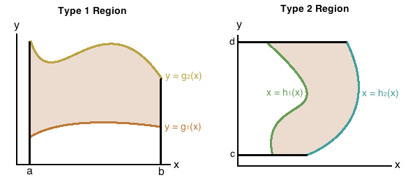
Procedure: Double Integral Over Region §

1. Sketch the functions and determine region type and which functions are above and below
2. Using the formula below, substitute the bounds of integration with the upper and lower functions respectively

$$\begin{array}{rl}\text{Type I}=& {\int }_a^b{\int }_{g_1(x)}^{g_2(x)}f(x,y)dydx\\ \text{Type II}=& {\int }_d^c{\int }_{h_1(x)}^{h_2(x)}f(x,y)dxdy\end{array}$$

Example: Double Integrals over Region

Evaluate $\int {\int }_D(2x+y)dA$ where $D$ is the region bounded between $x=y^2$ and $x=2-y$.

Double Integral in Polar §

• Simply convert all $\sqrt{x^2+y^2}$ into $r$

Change of Variables §

Motivation: Change of Variables §

• Integrating areas bounded by functions $f_1,f_2$ in Cartesian coordinates require that an function “upper” bounds a “lower” function
• However, this may be difficult for some regions; a region may be bounded by 2 functions, $f(x),g(x)$ where no function acts as the upper or lower bound over a certain domain, making it impossible to integrate in Cartesian system
• We use a transformation procedure to change our coordinate system to something more “convenient”, then apply a distortion factor to the result (Jacobian)
• What constitutes a convenient transformation?
  • Function is easier to integrate (becomes standard integrals)
  • Bounds are less complex

Procedure: Transformation §

• The formula for transformation is as follows

1. Find the functions bounding the desired region
2. The bounding functions will be your “canonical” $u,v$; manipulate the $u,v$ further so that they can represent $f(x,y)$ easily
3. Find the bounds for those functions
4. Compute the Jacobian (use sneaky trick)

$$\int {\int }_{x,y}f(x,y)dxdy=\int {\int }_{uv}\underset{f(x,y)\text{ written in terms of }u,v}{\underbrace{f(x(u,v),y(u,v)}})\cdot \frac{1}{\det \left[\begin{array}{cc}\frac{\partial u}{\partial x}& \frac{\partial u}{\partial y}\\ \frac{\partial v}{\partial x}& \frac{\partial v}{\partial y}\end{array}\right]}dudv$$

Sneaky Trick: Jacobian Reciprocal §

• The Jacobian is defined as

$$J=\det \left[\begin{array}{cc}\frac{\partial x}{\partial u}& \frac{\partial x}{\partial v}\\ \frac{\partial y}{\partial u}& \frac{\partial y}{\partial v}\end{array}\right]$$

• Often times we have $u,v$ written in terms of $x,y$, which means we can’t directly compute the Jacobian; we need to rewrite them in terms of $x,y$ which is time-intensive
• A trick is that the reciprocal of the Jacobian, with respect to $u,v$, is the same as the original Jacobian, that is

$$J=\frac{1}{\det \left[\begin{array}{cc}\frac{\partial u}{\partial x}& \frac{\partial u}{\partial y}\\ \frac{\partial v}{\partial x}& \frac{\partial v}{\partial y}\end{array}\right]}$$

Applications of Double Integrals §

Applications of double integral: mean value, mass, static moments, center of mass, moments of inertia)

Triple integral over a box. Fubini’s theorem application §

(Iterated integral)

Triple integral over a simple region §